How it works
Field boundaries
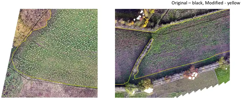
Whichever mapping tool is used to generate the KML file, the field boundaries need to be drawn correctly. The black line is not precise enough. The improved yellow outline ensures that the field areas are correct, and the algorithm knows where to look for plants, thus accelerating the analysis.
Orthorectification and slicing
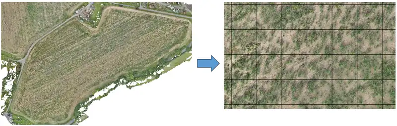
Orthorectification corrects geometric distortions in the aerial imagery. The result is an image that accurately represents the Earth’s surface as if viewed from directly overhead. This process removes distortions caused by camera tilt, terrain variations, and the curvature of the Earth, making the imagery suitable for accurate measurement and mapping. The complete picture of the surved field is then cut into equal-sized pieces, slices, which are then fed to gono.ai for analysis.
Detection of extents and centroids
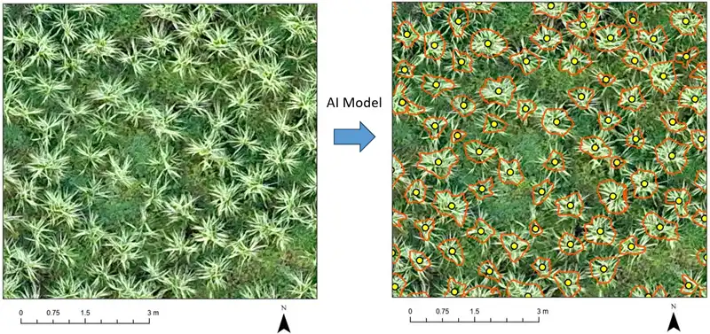
The algorithm scans these slices, distinguishing between the background (soil), weeds, and other plants different from Miscanthus, as well as other disturbances, in order to correctly identify the plant’s size, shape, and extent, as well as the point at which its stem emerges, or the plant’s centroid. In densely planted fields, or older fields (the image above is a 1st year field) the canopies of adjacent plants overlap, or a plant may be shorter and less visible amongst its taller neighbors. Thus, correctly identifying the plant’s center point and distinguishing it from weeds is important for an accurate plant count. This is where training the model is necessary for different genotypes or environmental conditions.
Example 1 – survey
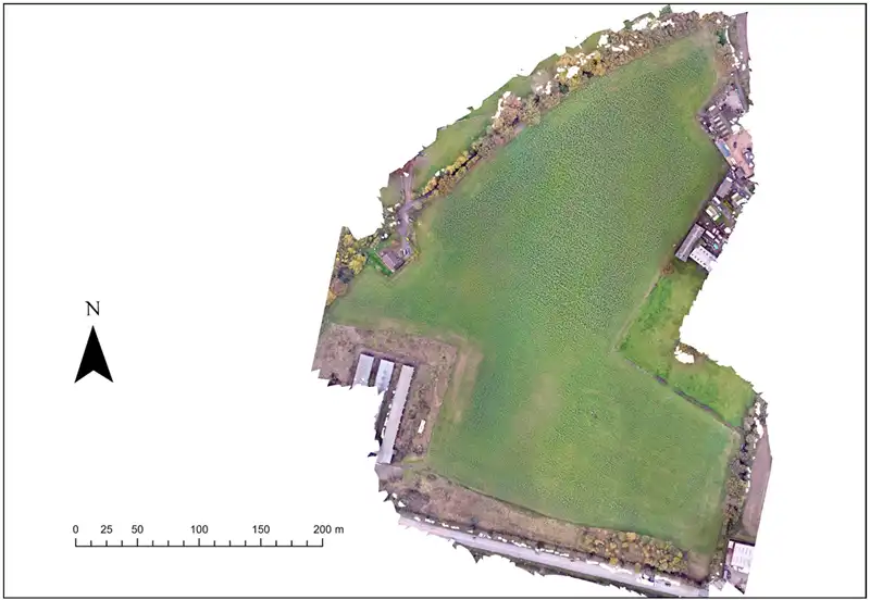
Due to very dry conditions right after planting, this Miscanthus grower wasn’t sure after the first nine months if his newly planted crop had achieved its target establishment percentage of at least 80% or 1.2 plants per square meter.
Example 1 – heatmap and benchmarking

His concerns were unfounded. Not only did his crop achieve 1.2 plants per square metre, but after the first year of establishment, the number of emerged plants surpassed that figure, reaching 1.3 plants per square metre — an excess of 8% over the target. Since Miscanthus grows its roots first, it is expected that this number will increase as more plants emerge in the second year. Therefore, the lighter green spots in the heat map will shrink or eventually disappear altogether.
Example 2 – survey
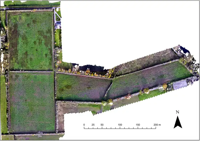
This grower planted Miscanthus on four adjacent fields that had never produced satisfactory yields of cash crops due to uneven soil conditions. Some areas had very shallow soil, while others had very heavy, nutrient-poor soil. Other areas were very sandy and prone to drought. The grower wanted to know if Miscanthus could withstand these conditions and how well it would fare.
Example 2 – survey
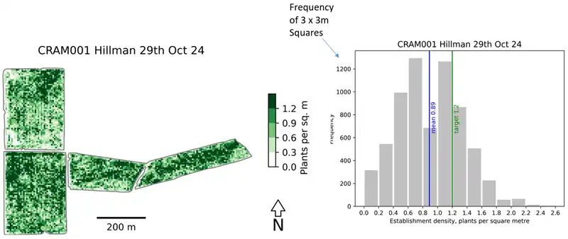
In this case, the uneven soil conditions are clearly evident in the establishment of the Miscanthus. After the first year, the threshold of 1.2 plants per square meter has not been reached. Although the density will surely increase in the second year of growth as more and more plants emerge. It is unlikely though that the 30% gap will be completely covered. Some areas, especially in the far right field, seem to be well covered. The top field, with its shallow soil conditions, presents difficulties not only for cash crops, but also for Miscanthus. Nevertheless, the crop will provide an acceptable return (with approx. 1 plant per square meter after the second year), allowing the grower to devote his time to his more productive fields instead of investing year after year in an area of his farm that simply doesn’t yield well.