Why drone surveys are required

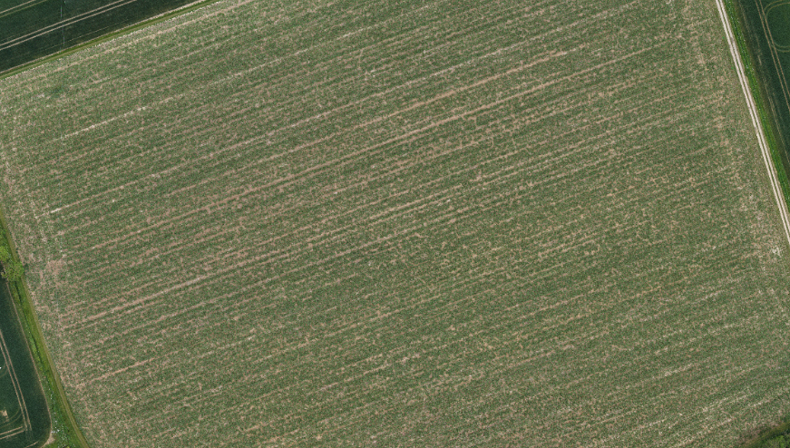
The aerial view of a second-year Miscanthus field after two months of growth: at this altitude, the crop appears uniform and promising.

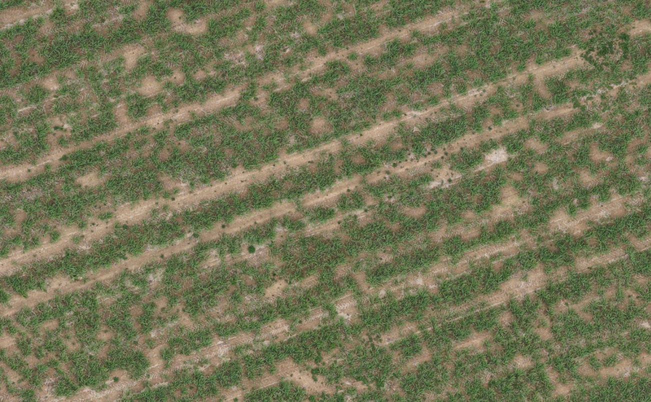
Taking a closer look reveals variation within the canopy. The rows are clearly distinguishable, as are some gaps within the same row.

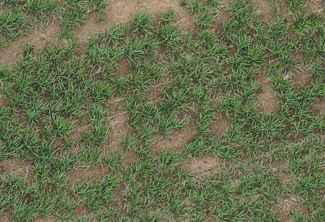
At ground level the truth becomes clear: local establishment quality varies considerably.

What AI-supported drone surveying reveals

By counting actual plant emergence against the number of rhizomes sown, gono.ai replaces guesswork with a precise figure: 13,532 plants emerged from 19,000 rhizomes planted, equal to an emergence rate of 71.22%.

That is an acceptable establishment rate, but 80% would have been achievable. That gap is not abstract: it means the current field will be operating below its potential yield by a difference of 8%. This deficit will compound every harvest season across a 20-year crop cycle.

A single extra day of field preparation before the next planting project could prove to be one of the highest-return investments of this farm.

AI-supported drone surveying in a nutshell

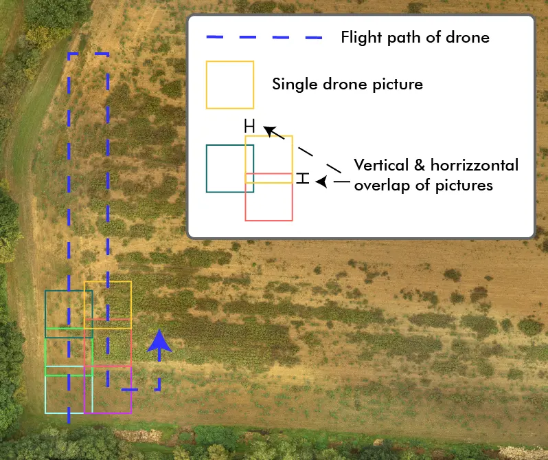
Please imagine taking a photograph of a field from above, with such high-quality detail that every single plant is clearly visible. Instead of taking a single image, a drone is flown over the field in a straight line, capturing a series of smaller photos along the way. Each photo is slightly overlapping the next.

The drone needs to fly at the right height so that each pixel in the photo matches a tiny square on the ground. This ensures the pictures are sharp enough for the AI to count individual plants. Also the drone’s flight path needs to be planned and set how often it takes a picture based on how fast it’s flying. There are apps and calculators to help figure this out.

Once the drone finishes its flight, the photos are stitched together seamlessly assembling the individual pieces into a unified whole to create a single, detailed map of the field. This map is then analysed by AI to count the plants.

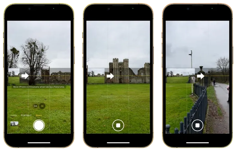
The concept is comparable to capturing a panorama using a mobile phone, but rather than photographing a wide landscape, gono.ai employs a high-resolution bird’s-eye view of the field. This method is most effective when the plants are well-grown and not excessively overlapping. Typically, this is the case after 2 to 3 months of growth following planting.

Precise field boundaries are important

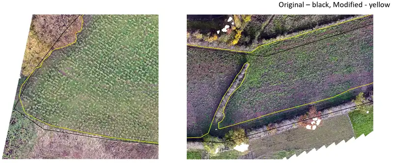
Whichever mapping tool is used to generate the KML file, the field boundaries need to be drawn correctly. The black line in the image above is not precise enough. The improved yellow outline ensures that the field areas are correct, and the algorithm knows where to look for plants, thus accelerating the analysis.

Digesting the survey: ortho-rectification and slicing

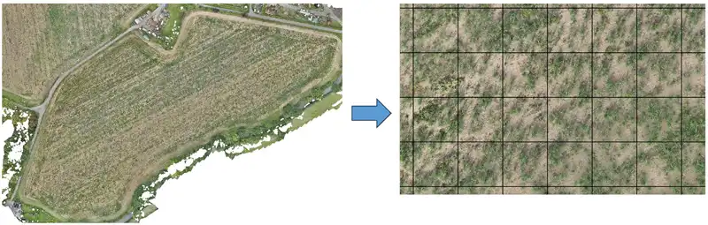
Orthorectification corrects geometric distortions in the aerial imagery. The result is an image that accurately represents the Earth’s surface as if viewed from directly overhead. This process removes distortions caused by camera tilt, terrain variations, and the curvature of the Earth, making the imagery suitable for accurate measurement and mapping. The complete picture of the surved field is then cut into equal-sized pieces, slices, which are then fed to gono.ai for analysis.

Analysis: detection of extents and centroids

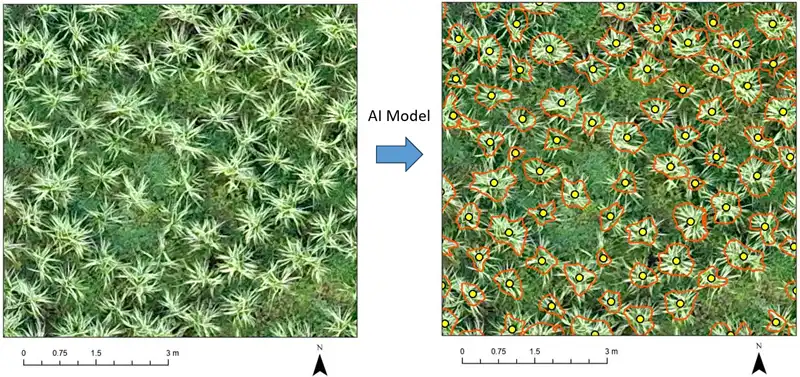
The algorithm then scans these slices, distinguishing between the background (soil, weeds and other plants different from Miscanthus) in order to correctly identify the plant’s size, shape and extent. The centre of this shape is then taken to be the point at which its stem emerges, or the plant’s centroid. In fields with dense plantations or those that are more mature, the canopies of the plants that are located adjacent to each other overlap.

Therefore, it is essential to correctly identify the plant’s centre point and differentiate it from weeds to ensure an accurate plant count. In this instance, it is essential to train the model for different genotypes or environmental conditions.

Example 1 – drone surveying

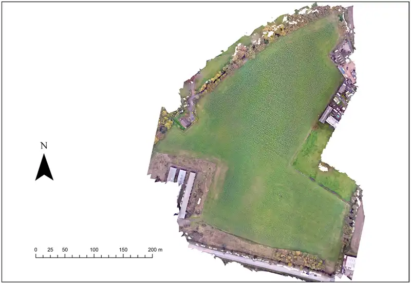
Due to very dry conditions right after planting, this Miscanthus grower wasn’t sure after the first nine months if his newly planted crop had achieved its target establishment percentage of at least 70% or 1.2 plants per square meter.

Example 1 – heatmap and benchmarking

His concerns were unfounded. Not only did his crop achieve 1.2 plants per square metre, but after the first year of establishment, the number of emerged plants surpassed that figure, reaching 1.3 plants per square metre — an excess of 8% over the target. Since Miscanthus grows its roots first, it is expected that this number will increase as more plants emerge in the second year. Therefore, the lighter green spots in the heat map will shrink or eventually disappear altogether.

Example 2 – drone surveying

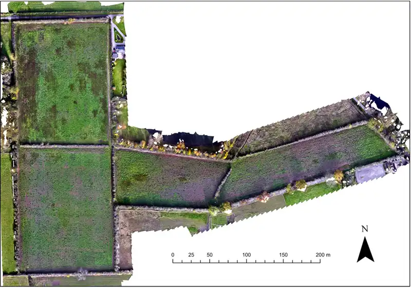
This grower planted Miscanthus on four adjacent fields that had never produced satisfactory yields of cash crops due to uneven soil conditions. Some areas had very shallow soil, while others had very heavy, nutrient-poor soil. Other areas were very sandy and prone to drought. The grower wanted to know if Miscanthus could withstand these conditions and how well it would fare.

Example 2 – survey

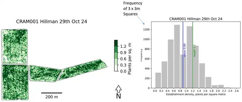
In this case, the uneven soil conditions are clearly evident in the establishment of the Miscanthus. After the first year, the target of 1.2 plants per square metre has not been reached. Although the density will increase in the second year of growth as more plants emerge, it is unlikely that the 30% gap will be fully closed. It appears that certain areas, notably those in the far right field, have been adequately covered. The top field, with its shallow soil conditions, poses challenges not only for cash crops but also for Miscanthus. Despite its versatility and ease of cultivation, Miscanthus requires a soil depth of at least 40 cm for successful establishment.

Nevertheless, the crop will provide a satisfactory return (with approximately 1 plant per square metre after the second year), allowing the grower to focus their time and resources on the more productive fields of their farm. This approach ensures that investment is focused on areas of higher yield, leading to more efficient use of time and financial resources.